Master These 5 Excel Hacks and Save Valuable Time

Microsoft Excel is a powerful tool, and it’s useful for more than numbers. Many people use Excel to manage tasks in their everyday lives beyond financial calculations.

Most Excel users aren’t aware of all the intricate tips and tricks that help you get the most out of Excel. There are so many functions and formulas to help you slice and dice numbers or give that data a new look, it’s impossible to recount them all.

We’ve put together a list of five of our favorite Excel hacks that can save you time, are easy to master, and impress your colleagues.

1. Flash Fill Your Data Just Like Magic

Want to manipulate your data as quick as a flash? Don’t rely on a complex combination of functions such as FIND, LEFT, CONCATENATE, or Text to Columns. Flash Fill is a powerful and time-saving tool that automatically fills your data when it senses a pattern.

Let’s say you have a list of GL accounting codes, and you want to extract the integer part of the code. Just complete the first cell, and Excel will generate a preview as you type to complete the list based on your provided pattern. Press Enter to accept the suggestion.

Just like magic, your data entry is complete and free from errors.

You can even use Flash Fill to combine and adjust your data.

To turn on Flash Fill go to File > Options > Advanced > Editing Options > select the Automatically Flash Fill box.

Or run it manually by clicking Data > Flash Fill, or use shortcut Ctrl+E.

Things to remember:

• Flash fill works best when the source data is consistent.
• Flash Fill is not dynamic, so if you change the source cell, the result doesn’t update automatically.
• To ensure that Flash Fill recognizes a pattern, you need to use Flash Fill close to the source data.

2. F2 is Not the Only Way to See Where That Number Came From

When you’re trying to work out exactly what is behind your profit and loss (P&L) figures (or any figure), you can read the formulas, and when you’re editing a cell, Excel has the good sense to highlight the precedent cells (the cells referred to in the selected cell).

Nice right?

Except when the spreadsheet is so complex that all the precedent cells are not visible in the same window. They could be anywhere. And then you have to go and find them. And you lose the other cells. And the source formula.

OR

Use Formula > Trace Precedents. Excel will draw some nice (persistent) arrows for you, from the selected cell to its precedents.

Or its dependents (the cells that depend on the cell you’re looking at) even!

And you can even select Trace Precedents or Trace Dependents again, to have arrows pointing at the precedents of the precedents for your cell

When you have covered your spreadsheet with little blue arrows, you can select Remove Arrows to clear the air.

If you haven’t already, give it a try. We’re sure you’ll love it.

You can even take it up a notch with some shortcuts:

• Press Ctrl+[ to go straight to the precedent cells
• Press Ctrl+] to go straight to the dependent cells
• Double-click on the dotted line to an off-sheet reference to go straight to it

3. Quickly See Insights Into Your Data With Conditional Formatting

Want quick insights into your data? Conditional Formatting on the Home ribbon can help you make sense of your data by highlighting trends or patterns in your data based on rules that you create.

You can apply conditional formatting to a range of cells, an Excel table, or even a PivotTable report. You can even apply multiple conditional formats to the same cells. Highlight the cells you want to format, and then try these options.

Option A. Click on the Quick Analysis button that appears next to your highlighted cells or Ctrl +Q to display the pop-up menu.

1. To see a live preview of your data with formatting applied, hover over the different options in the Formatting window. The formatting options differ depending on the type of data you have selected. For example, you’ll have different options if your data contains only text as opposed to text and numbers.
2. Click on the formatting option you want.

Note: If you change the data in a cell so that it satisfies the conditional formatting rules, the format automatically changes too.

Option B. If you want more control over what type and when conditional formatting applies, you can create your own rule. Use this option to format blank cells or error cells.

1. Go to Home > Conditional Formatting > New Rule.
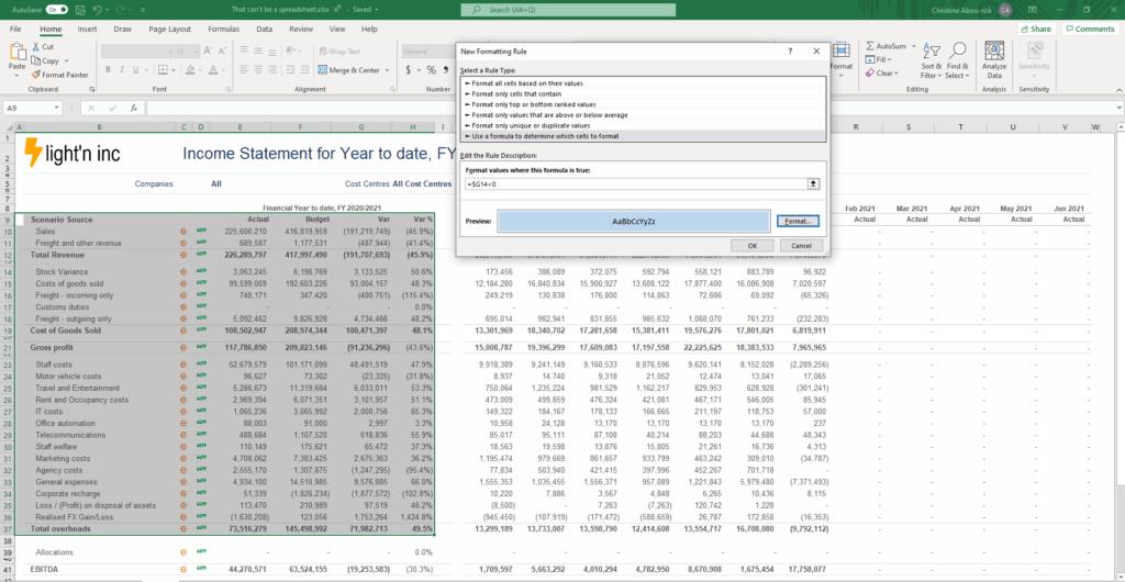
2. In the New Formatting Rule dialog box, select a Rule Type and then Edit the Rule Description to set your specific parameters.

In the following example, we have used a formula to highlight rows where our Actuals for Costs exceeded our Budget, by looking at whether the Variation column (column G) is negative. The rows where the formula G<0 is true, are highlighted.

The result of conditional formatting is below: 

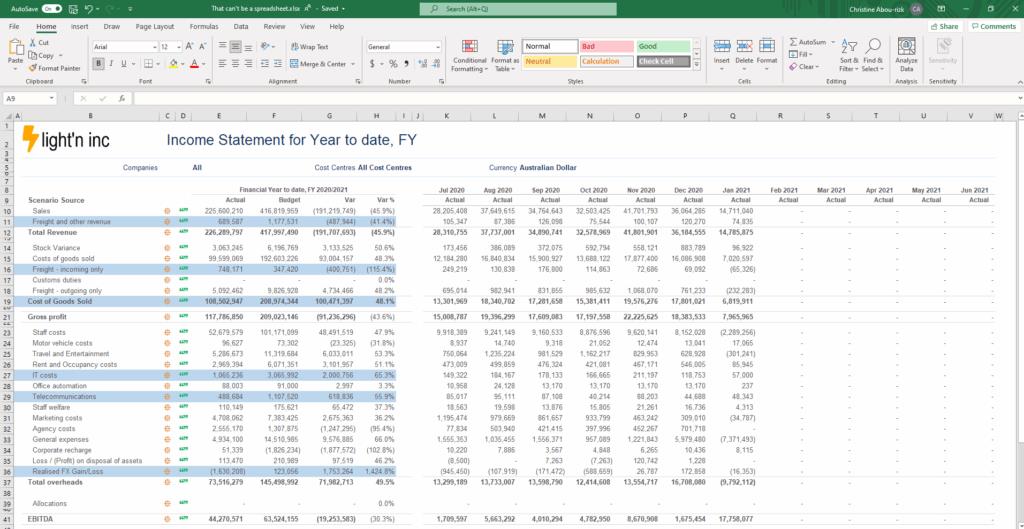
To present your data more clearly, you can also sort or filter your data based on conditional formatting.

4. Simplify Your Workbook by Hiding Data in Plain Sight

Hiding a row or column in Excel is simple—just select the whole column by clicking the letter (or number for row) header, right-click, and select “Hide.” You can unhide by selecting the columns to either side of the hidden column, right-clicking, and selecting “Unhide.”

But what if you have a section of inconveniently placed data you want to hide, but you still want to be able to work with?

1. Highlight the cells you want to hide > right-click > select Format Cells….
2. In the Number tab, select the Category type “Custom.”
3. In the Type field, input three semicolons ” ;;; ” and click OK.

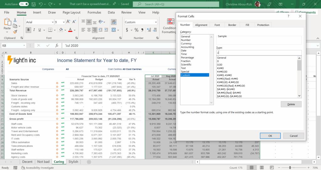
Now the numbers aren’t visible, but you can still use them in formulas. The values of these cells can be found in the preview area next to the Function button. You can take this hack even further.

When collaborating with a team or integrating data from different sources, your Excel workbook can get overloaded with several sheets (each indicated by a tab at the bottom). To simplify your workbook, you can hide sheets, making their data still available not only for reference, but also available to formulas on other sheets in the workbook.

1. At the bottom, click on the sheet tab you want to hide, then right-click on the sheet label and choose Hide.
2. To find it again, go to the Home ribbon, click Format, and hover over Visibility, Hide & Unhide. Click Unhide, pick the sheet name from the list of hidden sheets that pops up, and click OK.

5. Keep Your Data Clean With the Data Validation Function

We understand the importance of clean data, especially when you’re collaborating with teams across your organization. When you’re creating a spreadsheet for others to use, consider restricting what data users can input to ensure data entered is valid. Use Data Validation to restrict the type of data or the values that users enter into a cell. You can even create the error message they’ll see.

One of the most common data validation uses is to create a drop-down list:

1. Highlight the cells you want to create a rule for.
2. Go to the Data ribbon  and click on Data Validation, or use Alt > D > L keyed separately to open the Data Validation dialog box.
3. On the Settings tab, under Allow, select List for drop-down menu. Note that there are other options that allow you to restrict to whole number, decimal, date, time, or text length.
   
   
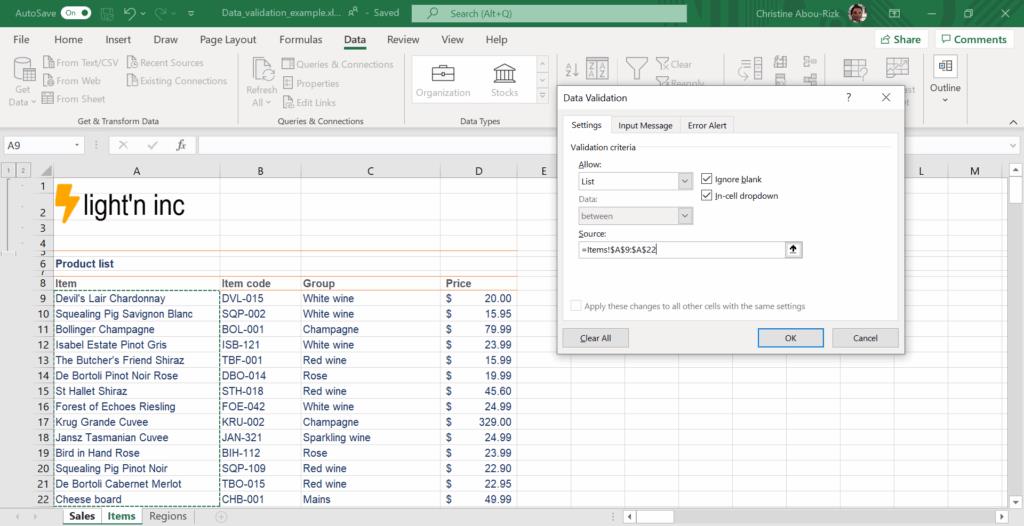
4. Click in the Source box, then either type a list, with commas between the options or click the button next to the Source field and then select your list range. You can also insert custom formulas, for example ISTEXT or ISNUMBER to restrict the type of data.
   Tip: Having your list items in an Excel table means that as you add or remove items from the list, any drop-downs you based on that table will automatically update.
5. Check the In-cell dropdown box.
6. Click the Input Message tab if you want a message to pop up when the cell is clicked. Check the Show input message when cell is selected box, and insert a title and message.
7. Click the Error Alert If you want a message to pop up when someone enters something that’s not in your list. Check the Show error alert after invalid data is entered box, pick an option from the Style box, and insert a title and message.
8. Click OK.

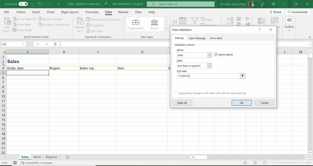
Another common user error is inputting a future date into a form or for a transaction. In this example, we prevent future dates from being entered into Excel by using the Data Validation function and TODAY formula.

1. Highlight the cell(s) you want to create a rule for.
2. Go to the Data ribbon and click Data Validation or use Alt > D > L keyed separately to open the Data Validation dialog box.
3. In the Settings tab, under Allow, select Date.
4. The Data field can be either less than or less than or equal to. This is essentially whether you want to include the present day in validation.
5. Enter an End Date of =TODAY() – this formula retrieves the present date.
6. Optional: Click the Error Alert tab and modify the error message.
7. Click OK button to apply the validation.

Note: Although you can enter any date into the End Date or any date-related field in the Data Validation dialog, using the TODAY formula makes the validation dynamic.

If you like the familiar feel of Excel and want to find out about more advanced ways to handle reporting and save time, explore our webinars.

Get Your Sheet Together: A Two-Part Webinar Series

Download Now:

"*" indicates required fields

This field is hidden when viewing the form

Select Your Closest Time Zone

-- Select One --

This field is hidden when viewing the form

Platform*

First ChoiceSecond ChoiceThird Choice

Use Case*

-- Select One --I'm a current user and updating my applicationI'm a current user and interested in expanding usageI'm new here and interested in evaluating

Business Email*

First Name*

Last Name*

Phone Number*

Company Name*

Job Title

This field is hidden when viewing the form

Industry

Primary Financial System

-- Select One --DeltekEpicorInforJD EdwardsMicrosoftMRI SoftwareNetSuiteOracleOtherSageSAPSYSPROViewpoint

Financial System Version

-- Select One --24SevenOfficeA+AAROAccountEdgeAccounting CSAccountmateAcumaticaAlereAnaplanApteanAssistASWAurora (Sys21)AxionAxisBAANBannerBlackbaudBlueLinkBook WorksBPCSCayentaCCHCDK GlobalCedAr e-financialsCGI AdvantageClarusCMiCCMS (Solarsoft)CodaCoinsColleagueCPSICSC CorpTaxCustomCYMADACData WarehouseDatatelDATEVDavisware Global EdgeDavisware S2KDeacomDeltek AjeraDeltek ComputerEaseDeltek CostPointDeltek MaconomyDeltek VantagePointDeltek VisionDeltek Vision CloudDPNDynamics 365 Business CentralDynamics 365 Finance and Supply Chain ManagementDynamics AXDynamics CRMDynamics GPDynamics NAVDynamics NAV C5Dynamics SLe5eCMSEden (Tyler Tech)EmphasysEntrataEpicor AvanteEpicor BisTrackEpicor CMSEpicor EnterpriseEpicor Epicor SLSEpicor iScalaEpicor KineticEpicor LumberTrackEpicor Manage 2000Epicor Prophet 21Epicor TroposEtailExpandableFAMISFamous SoftwareFernFinancialForceFireStreamFISFiServFlexiFortnoxFoundationFourth ShiftFriedmanFull CircleGEMSHarris Data (AS/400)HCSHMSIBM Cognos TM1IBSIBS-DWIn-House DevelopedIncodeINFINIUMInfor CloudSuite FinancialsInfor Distribution SX.eInfor Financials & Supply ManagementInfor LawsonInfor M3Infor System21Infor SyteLineIQMSiSuiteJack HenryJenzabarJobBOSSJonas ConstructionM1MacolaMACPACMade2ManageMAMMAM AutopartManmanMapicsMcLeodMEDITECHMFG ProMicrosOperaMIPMitchell HumphreyMovexMRIMRI Commercial ManagementMRI FinancialsMRI HorizonMRI Horizon CREMRI Qube HorizonMRI Residential ManagementMSGovernMunis (Tyler Tech)New World SystemsOnesiteOnestream XFOpen SystemsOracle E-Business Suite (EBS)Oracle EPM CloudOracle ERP CloudOracle EssbaseOracle Financial Consolidation and Close (FCCS)Oracle FusionOracle Hyperion EnterpriseOracle Hyperion Financial Management (HFM)Oracle Hyperion PlanningOracle PeopleSoftOracle Planning and Budgeting Cloud Service (PBCS)Oracle Tax ReportingPDIPentaPlexxisPowerOfficePRMSPro ContractorProLawQ360QADQuantumQube HorizonQuickBooks Desktop PremierQuickBooks Desktop ProQuickbooks EnterpriseQuickBooks OnlineQuorumRealPageREST APIRetalixRossSage 100Sage 100 ContractorSage 200Sage 300Sage 300 CRE (Timberline)Sage 500Sage 50cloud AccountingSage AccPacSage Adonix TolasSage EstimatingSage IntacctSage Intacct Budgeting & PlanningSage MASSage X3SAP BPC (HANA, MS or Netweaver)SAP Business ByDesignSAP Business One (B1)SAP Business Warehouse (BW)SAP ERPSAP ERP Central Component (ECC)SAP S/4HANASmartStreamSpokaneSpringbrookSQL Server Analysis Services (SSAS)Standalone DB with ODBC/DSN connectionStandalone IBM DBStandalone Oracle DBStandalone SQL DBSUNSunguardSunSystemsSys21SyteLineTAM (Applied Systems)Thomson Reuters TaxTimberlineTIMELINETraverseTripleTexUnit4Unit4 AgressoUnit4 Business WorldUnit4 CodaUSL FinancialsVadimVAI-System 2000VantageVertexViewpoint SpectrumViewpoint VistaVismaWinshuttleWolters Kluwer CCH TagetikWorkDayXeroxLedgerXperiaYardiYardi-SaaS

This field is hidden when viewing the form

Current ERP Implementation Partner

Product of Interest

-- None --Agility PIMAnglesAngles Enterprise for Oracle- Reporting for OracleAngles Enterprise for SAPAngles ProfessionalAtlasBizNetBizviewCalumoCertent- Certent Disclosure Management- Certent DisclosureNet- Certent Equity ManagementClausion Consolidation- TabellaCubewareCXODundas BIESGEvent 1 SoftwareExagoEZLease- EZLease LessorFiplanaFXLoaderHubbleIDL- IDL Cockpit- IDL Designer- IDL Forecast- IDL Konsis- IDL PublisherIzendaJet- Jet Analytics- Jet Basics- Jet ReportsJustPerformKalidoLease ControllerLeaseAcceleratorLegerity Financials- FastPostLogi ComposerLogi InfoLogi ReportLogi SymphonyLongview- Longview Analytics- Longview Close- Longview Plan- Longview Tax- Longview Transfer PricingMekko GraphicsPower ON- Power ON Budget PlannerProcess Runner- Financial Optimization for SAPProcess Runner GLSUPureLeaseReal Estate ManagerSimba- Simba Drivers- Simba Managed Services- Simba SDKSourceConnectSpreadsheet ServerTidemarkViareport- Viareport Consolidation- Viareport LeaseVizlibWands- Wands for Oracle- Wands for SAPWrite!

BI Tool

TableauPower BIQlikLookerDomoAWS - QuickSightThoughtSpotCustom BuildOther

This field is hidden when viewing the form

What is your biggest challenge within your financial department?

This field is hidden when viewing the form

What is your primary reason for attending?

-- Select One --Researching this topicEvaluating software solutionsExisting customer or partner

This field is hidden when viewing the form

Which solutions are you currently evaluating?

-- Select One --Accounting & TreasuryAutomation & Data ManagementBudgeting & PlanningClose & ConsolidationEmbedded AnalyticsFinancial ReportingOperational Reporting & AnalyticsTax & Compliance

This field is hidden when viewing the form

Seniority

This field is hidden when viewing the form

Role

This field is hidden when viewing the form

Sub Role

Country

-- Select --AfghanistanAlbaniaAlgeriaAmerican SamoaAndorraAngolaAntigua and BarbudaArgentinaArmeniaAustraliaAustriaAzerbaijanBahamasBahrainBangladeshBarbadosBelarusBelgiumBelizeBeninBermudaBhutanBoliviaBosnia and HerzegovinaBotswanaBrazilBruneiBulgariaBurkina FasoBurundiCambodiaCameroonCanadaCape VerdeCayman IslandsCentral African RepublicChadChileChinaColombiaComorosCongo, Democratic Republic of theCongo, Republic of theCosta RicaCroatiaCubaCuraçaoCyprusCzech RepublicDenmarkDjiboutiDominicaDominican RepublicEcuadorEgyptEl SalvadorEquatorial GuineaEritreaEstoniaEthiopiaFaroe IslandsFijiFinlandFranceFrench PolynesiaGabonGambiaGeorgiaGermanyGhanaGreeceGreenlandGrenadaGuamGuatemalaGuineaGuinea-BissauGuyanaHaitiHondurasHong KongHungaryIcelandIndiaIndonesiaIranIraqIrelandIsraelItalyJamaicaJapanJordanKazakhstanKenyaKiribatiKosovoKuwaitKyrgyzstanLaosLatviaLebanonLesothoLiberiaLibyaLiechtensteinLithuaniaLuxembourgNorth MacedoniaMadagascarMalawiMalaysiaMaldivesMaliMaltaMarshall IslandsMauritaniaMauritiusMexicoMicronesiaMoldovaMonacoMongoliaMontenegroMoroccoMozambiqueMyanmarNamibiaNauruNepalNetherlandsNew ZealandNicaraguaNigerNigeriaNorth KoreaNorthern Mariana IslandsNorwayOmanPakistanPalauPalestine, State ofPanamaPapua New GuineaParaguayPeruPhilippinesPolandPortugalPuerto RicoQatarRomaniaRussiaRwandaSaint Kitts and NevisSaint LuciaSaint Vincent and the GrenadinesSamoaSan MarinoSao Tome and PrincipeSaudi ArabiaSenegalSerbiaSeychellesSierra LeoneSingaporeSint MaartenSlovakiaSloveniaSolomon IslandsSomaliaSouth AfricaSouth KoreaSpainSri LankaSudanSudan, SouthSurinameSwazilandSwedenSwitzerlandSyriaTaiwanTajikistanTanzaniaThailandTogoTongaTrinidad and TobagoTunisiaTurkeyTurkmenistanTuvaluUgandaUkraineUnited Arab EmiratesUnited KingdomUnited StatesUruguayUzbekistanVanuatuVenezuelaVietnamVirgin Islands, BritishVirgin Islands, U.S.YemenZambiaZimbabwe

State/Province

-- Select State --AlabamaAlaskaArizonaArkansasCaliforniaColoradoConnecticutDelawareDistrict of ColumbiaFloridaGeorgiaHawaiiIdahoIllinoisIndianaIowaKansasKentuckyLouisianaMaineMarylandMassachusettsMichiganMinnesotaMississippiMissouriMontanaNebraskaNevadaNew HampshireNew JerseyNew MexicoNew YorkNorth CarolinaNorth DakotaOhioOklahomaOregonPennsylvaniaRhode IslandSouth CarolinaSouth DakotaTennesseeTexasUtahVermontVirginiaWashingtonWest VirginiaWisconsinWyoming-- Select Province --AlbertaBritish ColumbiaManitobaNew BrunswickNewfoundland and LabradorNova ScotiaNorthwest TerritoriesNunavutOntarioPrince Edward IslandQuebecSaskatchewanYukon

I agree to receive digital communications from insightsoftware and its partners (click here for full list of partners) containing news, product information, promotions, or event invitations. I understand that I can withdraw my consent at any time. Privacy Policy.

I'd also like to see a demo of insightsoftware solutions

This field is hidden when viewing the form

Hidden Fields

This field is hidden when viewing the form

Partner Referral

This field is hidden when viewing the form

Referral URL

This field is hidden when viewing the form

First Click URL

This field is hidden when viewing the form

Content Type dataLayer

This field is hidden when viewing the form

Pardot Visitor ID

This field is hidden when viewing the form

Google Client ID

This field is hidden when viewing the form

Google Click ID

This field is hidden when viewing the form

Experiment ID

This field is hidden when viewing the form

Experiment ID & Variant

This field is hidden when viewing the form

dataLayer Form Type

This field is hidden when viewing the form

Is Google Experiment

This field is hidden when viewing the form

Salesforce Campaign

This field is hidden when viewing the form

DemandBase SID

Company Type

This field is hidden when viewing the form

Employee Count

This field is hidden when viewing the form

Annual Revenue

This field is hidden when viewing the form

Annual Revenue Bucket

This field is hidden when viewing the form

3rd Party Company Name

This field is hidden when viewing the form

3rd Party Industry

This field is hidden when viewing the form

3rd Party Sub Industry

This field is hidden when viewing the form

3rd Party Employee Range

This field is hidden when viewing the form

3rd Party Revenue Range

This field is hidden when viewing the form

3rd Party Street Address

This field is hidden when viewing the form

3rd Party Data Source

This field is hidden when viewing the form

3rd Party Country

This field is hidden when viewing the form

3rd Party Primary SIC

This field is hidden when viewing the form

3rd Party Watch List Account Type

This field is hidden when viewing the form

3rd Party Watch List Account Status

This field is hidden when viewing the form

3rd Party Watch List Campaign Code

This field is hidden when viewing the form

3rd Party Watch List Account Owner

This field is hidden when viewing the form

3rd Party Primary NAICS

This field is hidden when viewing the form

3rd Party Website

This field is hidden when viewing the form

Create MQL Task

Comments

This field is for validation purposes and should be left unchanged.

Access Resource

Having trouble?

Cookies are required to submit forms on this website. Enable cookies. How insightsoftware is using cookies.

Still experiencing an issue? Please contact our website administration team.

Δ

The post Master These 5 Excel Hacks and Save Valuable Time appeared first on insightsoftware.